Get Started
What is Evidently?
Welcome to the Evidently documentation.
Evidently helps evaluate, test, and monitor data and AI-powered systems.
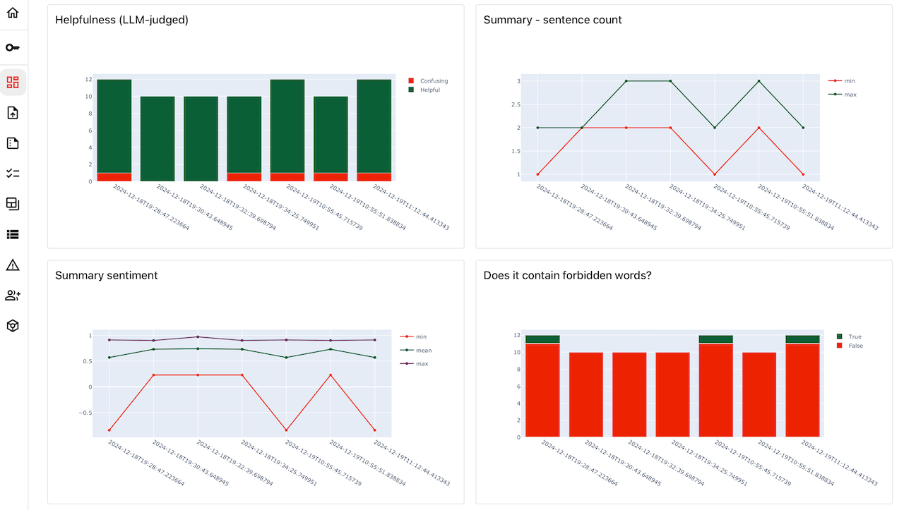
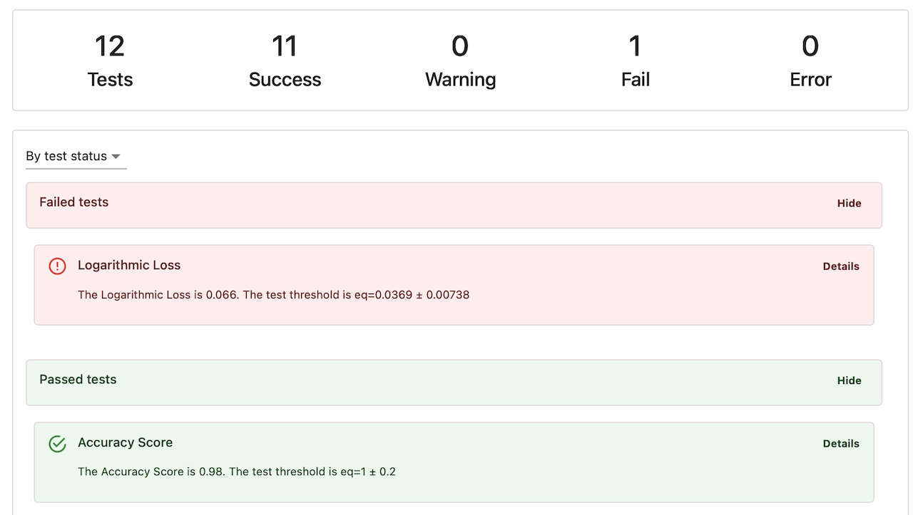
- Evidently is an open-source Python library with over 25 million downloads. It provides 100+ evaluation metrics, a declarative testing API, and a lightweight visual interface to explore the results.
- Evidently Cloud platform offers a complete toolkit for AI testing and observability. It includes tracing, synthetic data generation, dataset management, eval orchestration, alerting and a no-code interface for domain experts to collaborate on AI quality.
Our goal is to help teams build and maintain reliable, high-performing AI products: from predictive ML models to complex LLM-powered systems.
Get started
Run your first evaluation in a couple of minutes.
LLM evaluation
Evaluate the quality of LLM system outputs.
ML monitoring
Test tabular data quality and data drift.
Feature overview
What you can do with Evidently.
Evidently Platform
Key features of the AI observability platform.
Evidently library
How the Python evaluation library works.